num2vec: Numerical Embeddings from Deep RNNs

Categories Deep Learning, Machine Learning

Introduction

Encoding numerical inputs for neural networks is difficult because the representation space is very large and there is no easy way to embed numbers into a smaller space without losing information. Some of the ways to currently handle this is:

  • Scale inputs from minimum and maximum values to [-1, 1]
  • One hot for each number
  • One hot for different bins (e.g. [0-0], [1-2], [3-7], [8 – 19], [20, infty])

In small integer number ranges, these methods can work well, but they don’t scale well for wider ranges. In the input scaling approach, precision is lost making it difficult to distinguish between two numbers close in value. For the binning methods, information about the mathematical properties of the numbers such as adjacency and scaling is lost.

The desideratum of our embeddings of numbers to vectors are as follows:

  • able to handle numbers of arbitrary length
  • captures mathematical relationships between numbers (addition, multiplication, etc.)
  • able to model sequences of numbers

In this blog post, we will explore a novel approach for embedding numbers as vectors that include these desideratum.

Approach

My approach for this problem is inspired by word2vec but unlike words which follow the distributional hypothesis, numbers follow the the rules of arithmetic. Instead of finding a “corpus” of numbers to train on, we can generate random arithmetic sequences and have our network “learn” the rules of arithmetic from the generated sequences and as a side effect, be able to encode numbers as vectors and  sequences as vectors.

Problem Statement

Given a sequence of length n integers \(x_1, x_2 \ldots x_n\), predict the next number in the sequence \(x_{n+1}\).

Architecture

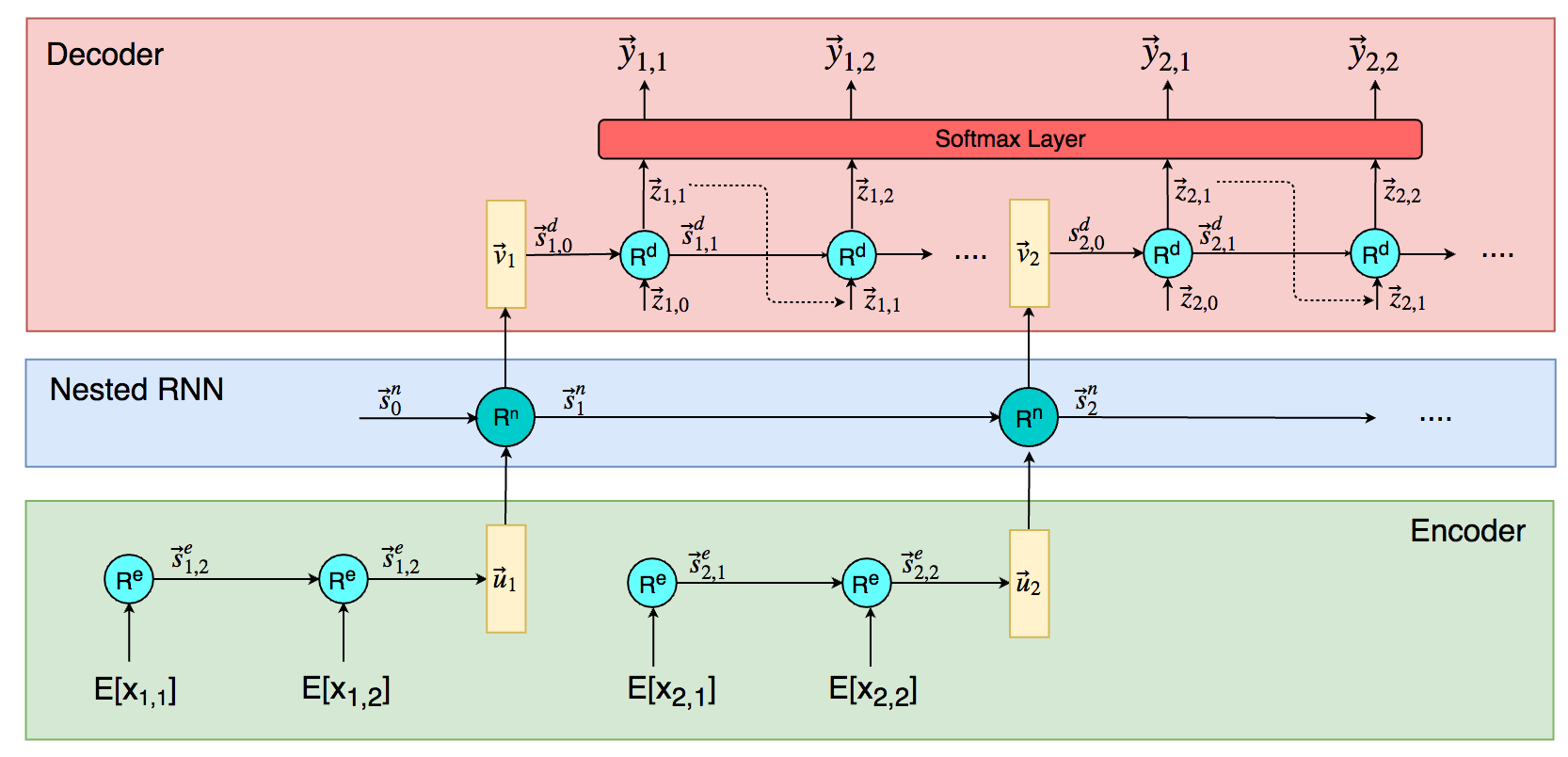
The architecture of the system consists of three parts: the encoder, the decoder and the nested RNN.

The encoder is an RNN that takes a number represented as a sequence of digits and encodes it into a vector that represents an embedded number.

The nested RNN takes the embedded numbers and previous state to output another embedded vector that represents the next number.

The decoder then takes the embedded number and unravels it through the decoder RNN to output the digits of the next predicted number.

Formally:

Let \(X\) represent a sequence of natural numbers where \(X_{i,j}\) represents the j-th digit of the i-th number of the sequence. We also append an <eos> “digit” to the end of each number to signal the end of the number. For the sequence X = 123, 456, 789, we have \(X_{1,2} = 2, X_{3,3} = 9, X_{3,4} = <eos>\).

Let \(l_i\) be the number of digits in the i-th number of the sequence (including <eos> digit. Let \(E\) be an embedding matrix for each digit.

Let \(\vec{u}_i\) be an embedding of the i-th number in a sequence. It is computed as the final state of the encoder. Let \(\vec{v}_i\) be an embedding of the predicted (i+1)-th number in a sequence. It is computed from the output of the nested RNN and used as the initial state of the decoder.

Let \(R^e, R^d, R^n\) be the functions that gives the next state for the encoder, decoder and nested RNN respectively. Let \(O^d, O^n\) be the functions that gives the output of the current state for the decoder and nested RNN respectively.

Let \(\vec{s}^e_{i,j}\) be the state vector for \(R^e\) for the j-th timestep of the i-th number of the sequence. Let \(\vec{s}^d_{i,j}\) be the state vector for \(R^d\) for the j-th timestep of the i-th number of the sequence. Let \(\vec{s}^n_i\) represent the state vector of \(R^n\) for the i-th timestep.

Let \(z_{i,j}\) be the output of \(R^d\) at the j-th timestep of the i-th number of the sequence.

Let \(\hat{y}_{i,j}\) represent the distribution of digits for the prediction of the j-th digit of the (i+1)th number of the sequence.

\(\displaystyle{\begin{eqnarray}\vec{s}^e_{i,j} &=& R^e(E[X_{i,j}], \vec{s}^e_{i, j-1})\\\vec{u}_i &=& \vec{s}^e_{i,l_i}\\ \vec{s}^n_i &=& R^n(\vec{u}_i, \vec{s}^n_{i-1})\\\vec{v_i} &=& O^n(\vec{s}^n_i)\\ \vec{z}_{i,j} &=& O^d(\vec{s}^d_{i,j})\\ \vec{s}^d_{i, j} &=& R^d(\vec{z}_{i,j-1}, \vec{s}^d_{i, j-1})\\ \hat{y}_{i,j} &=& \text{softmax}(\text{MLP}(\vec{z}_{i,j}))\\ p(X_{i+1,j})=k |X_1, \ldots, X_i, X_{i+1, 1}, \ldots X_{i+1, j-1}) &=& \hat{y}_{i,j}[k]\end{eqnarray}}\)

We use a cross-entropy loss function where \(y_{i,j}[t]\) represents the correct digit class for \(y_{i,j}\):

\(\displaystyle{\begin{eqnarray}L(y, \hat{y}) &=& \sum_i \sum_j -\log \hat{y}_{i,j}[t]\end{eqnarray} }\)

Since I also find it difficult to intuitively understand what these sets of equations mean, here is a clearer diagram of the nested network:
Training

The whole network is trained end-to-end by generating random mathematical sequences and predicting the next number in the sequence. The sequences generated contains addition, subtraction, multiplication, division and exponents. The sequences generated also includes repeating series of numbers.

After 10,000 epochs of 500 sequences each, the networks converges and is reasonably able to predict the next number in a sequence. On my Macbook Pro with a Nvidia GT750M, the network implemented on Tensorflow took 1h to train.

Results

Taking a look at some sample sequences, we can see that the network is reasonably able to predict the next number.

Seq [43424, 43425, 43426, 43427]
Predicted [43423, 43426, 43427, 43428]
Seq [3, 4, 3, 4, 3, 4, 3, 4, 3, 4]
Predicted [9, 5, 4, 3, 4, 3, 4, 3, 4, 3]
Seq [2, 4, 8, 16, 32, 64, 128]
Predicted [4, 8, 16, 32, 64, 128, 256]
Seq [10, 9, 8, 7, 6, 5, 4, 3]
Predicted [20, 10, 10, 60, 4, 4, 3, 2]

With the trained model, we can compute embeddings of individual numbers and visualize the embeddings with the t-sne algorithm.
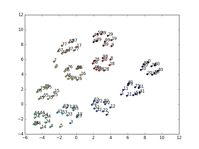
We can see an interesting pattern when we plot the first 100 numbers (color coded by last digit). Another interesting pattern to observe is within clusters, the numbers also rotate clockwise or counterclockwise.

We can also trace the path of the embeddings sequentially, we can see that there is some structure to the positioning of the numbers.
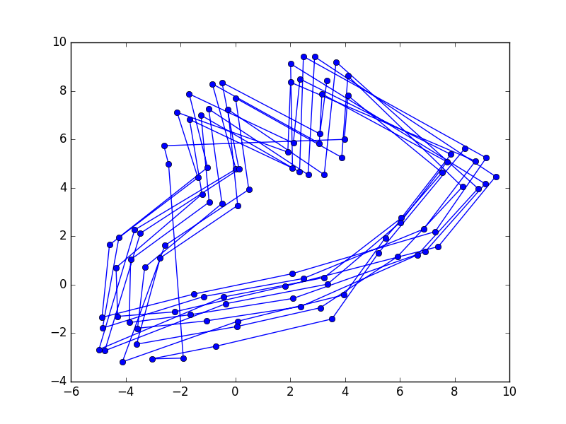
If we look at the visualizations of the embeddings for numbers 1-1000 we can see that the clusters still exist for the last digit (each color corresponds to numbers with the same last digit)
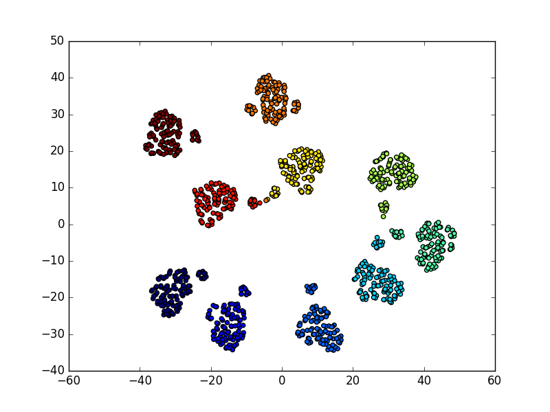
We can also see the same structural lines for the sequential path for numbers 1 to 1000:
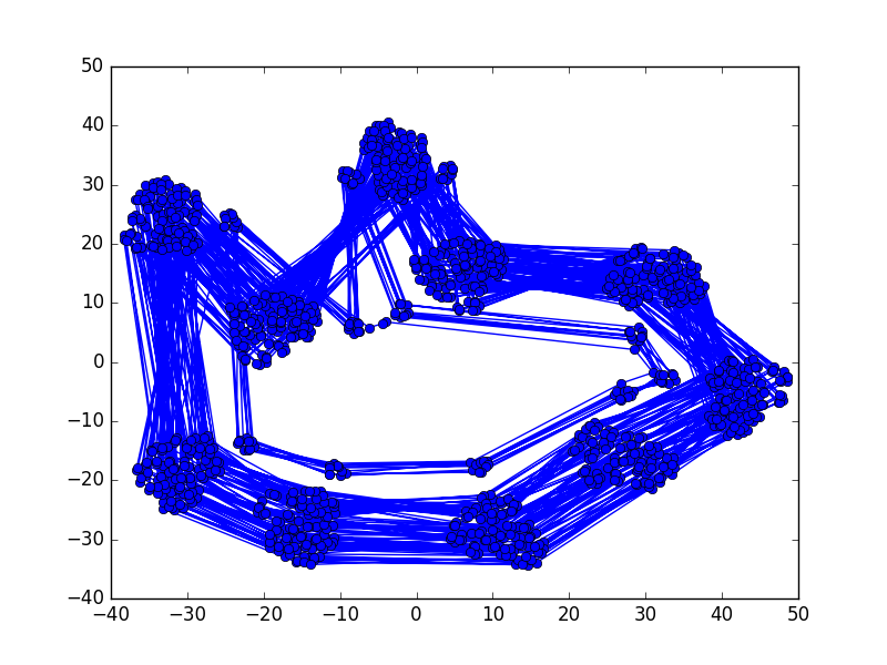
The inner linear pattern is formed from the number 1-99 and the outer linear pattern is formed from the numbers 100-1000.

We can also look at the embeddings of each sequence by taking the vector \(\vec{s}^n_k\) after feeding in k=8 numbers of a sequence into the model. We can visualize the sequence embeddings with t-sne using 300 sequences:
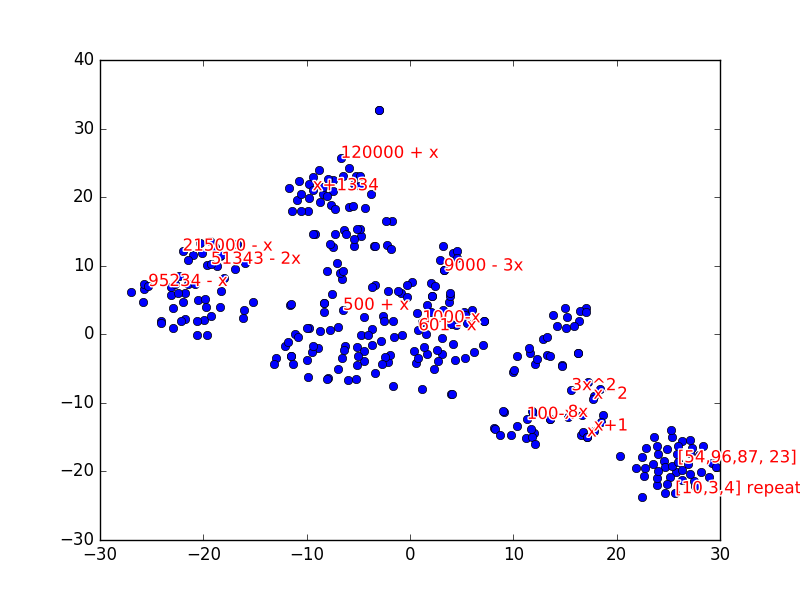
From the visualization, we can see that similar sequences are clustered together. For example, repeating patterns, quadratic sequences, linear sequences and large number sequences are grouped together. We can see that the network is able to extract some high level structure for different types of sequences.

Using this, we can see that if we encounter a sequence we can’t determine a pattern for, we can find the nearest sequence embedding to approximate the pattern type.

Code: Github

The model is written in Python using Tensorflow 1.1. The code is not very well written due to the fact that I was forced to use an outdated version of TF with underdeveloped RNN support because of OS X GPU compatibility reasons.

The code is a proof of a concept and comes from the result of stitching together outdated tutorials together.

Further improvements:

  • bilateral RNN
  • stack more layers
  • attention mechanism
  • beam search
  • negative numbers
  • teacher forcing


Tutorial: Getting Started with Distributed Deep Learning with Caffe on Windows

Categories Machine Learning, Uncategorized

Introduction

What is Caffe?

A deep learning framework developed by Berkeley Vision and Learning Center. It makes creating deep neural networks easy without writing a ton of code.If you don’t know what deep learning is, here is a great guide to getting started: http://cs231n.github.io/.

Setup

My setup:
Windows 8.1 on 64bit
Visual Studio 2013 Community
GeForce GT 750M
CUDA 7.5

1. Check for Compatibility

Make sure you are on a supported Windows operating system:
Windows 8.1
Windows 7
Windows Server 2008
Windows Server 2012.(If you are using Windows 8, upgrade through here: http://windows.microsoft.com/en-ca/windows-8/update-from-windows-8-tutorial)

Make sure your GPU is supported by CUDA: https://developer.nvidia.com/cuda-gpus 
Anything with compute capability of  >=3.0 should be good.

If you do not have a compatible GPU, you can still use Caffe but it will be magnitudes slower than with a GPU and skip part 2.

Make sure you have a compatible Visual Studios for CUDA support: 
Visual Studio 2013
Visual Studio 2013 Community (Download Visual Studio 2013 Community Edition Free)
Visual Studio 2012
Visual Studio 2010

More nVidia documentation at:
http://docs.nvidia.com/cuda/cuda-getting-started-guide-for-microsoft-windows/#axzz3wsl3JktL 

2. Install CUDA

Download and install CUDA toolkit here: https://developer.nvidia.com/cuda-downloads
 
Verify CUDA can compile:
Go to C:ProgramDataNVIDIA CorporationCUDA Samplesv7.5 and open the solution file (i.e. Samples_vs2013.sln) in Visual Studio
In the solution explorer, build 0_Simple/vectorAdd
Run C:ProgramDataNVIDIA CorporationCUDA Samplesv7.5binwin64debugvectorAdd.exe
 
The output should be:
Copy input data from the host memory to the CUDA device
CUDA kernel launch with 196 blocks of 256 threads
Copy output data from the CUDA device to the host memory
Test PASSED
Done

3. Install Caffe

Fork the windows port of Caffe: https://github.com/happynear/caffe-windowsDownload third party libraries and extract to caffe-windows/3rdparty
Remember to add caffe-windows/3rdparty/bin to your PATH

Open caffe-windows/buildVS2013/MainBuilder.sln in Visual Studio
If you don’t have a compatible GPU, open caffe-windows/build_cpu_only/MainBuilder.sln

Set the GPU compatible mode:
Right click the caffe project and click properties
In the left menu, go to Configuration Properties -> Cuda C/C++ -> Device
In the Code Generation key, modify the compute capabilities to your GPU’s (such as compute_30,sm_30; etc)

Build the solution in release mode
Right click the solution and click Build Solution
(It’s OK if matcafe and pycafe fail)

Testing
Download the mnist leveldb from http://pan.baidu.com/s/1mgl9ndu
Extract the folders to caffe-windows/examples/mnist
Run caffe-windows/run_mnist.bat

You should get some output similar to the following when you finish:
….
I0112 00:06:37.180341 45040 solver.cpp:326] Iteration 10000, loss = 0.00428135
I0112 00:06:37.181342 45040 solver.cpp:346] Iteration 10000, Testing net (#0)
I0112 00:06:51.726634 45040 solver.cpp:414]     Test net output #0: accuracy = 0
.9914
I0112 00:06:51.726634 45040 solver.cpp:414]     Test net output #1: loss = 0.027
0199 (* 1 = 0.0270199 loss)
I0112 00:06:51.726634 45040 solver.cpp:331] Optimization Done.
I0112 00:06:51.726634 45040 caffe.cpp:215] Optimization Done.

Full instructions can be found on the readme of https://github.com/happynear/caffe-windows

Results:
solver_mode: GPU
Start Time: 23:25:19.38
Finish Time: 23:28:37.62

solver_mode: CPU

Start Time: 23:38:01.62
Finish Time:  0:06:51.91As you can see, even a low-end GPU can train a magnitude faster than a CPU.

A Simple Artificial Intelligence Capable of Basic Reading Comprehension

Categories Machine Learning, Uncategorized
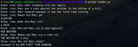
I was interested in an artificial intelligence that could do reading comprehension, but surprisingly,  I could not find much on the topic. I decided to try and create an AI that could do some basic reading comprehension and I got some good results:

Short Passage (Input):
Mary went sledding with her family. Mary won a race against her brother to the bottom of a hill. Mary cheered because it was her first time winning.

Input: Where did Mary go?
Output: Sledding

Input: What did Mary win?
Output: A race


Input: Who did Mary win a race against?
Output: Her brother

Input: Where did Mary win a race to?
Output: The bottom of the hill


Input: Why did Mary cheer?
Output: Because it was her first time winning


As we can see, the program can actually answer the questions about the passage.

Full Source Available Here

Introduction

What I am trying to accomplish is program capable of artificial semantic memory. Semantic memory refers to how we store our explicit knowledge and facts about the world. For example, our memory of our birth date or our knowledge that humans are mammals. I wanted to be able to make something that was able to read a passage and answer any questions I had.

Abstract Idea

An abstract idea of how I accomplished artificial semantic memory was to create a structure that can store a sentence in a different way that can be used to answer questions.

1. Structure the relationships betweens objects (nouns) in the sentence.

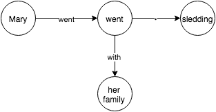
For example, in the sentence “Mary went sledding with her family”, there are three objects “Mary”, “sledding” and “her family”. Mary has a verb “go” (present tense of went) with the object “sledding”. The verb “go” is “with” the object “her parents”. 
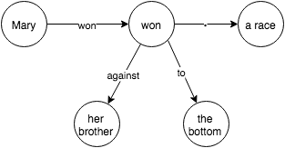
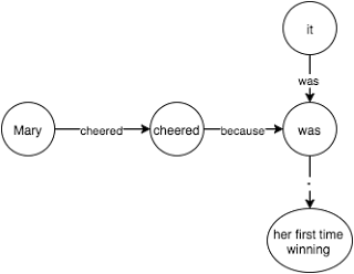
After brainstorming different ways to represent the relationships between objects and actions, I came up with a structure similar to a trie which I will call a “word graph”. In a word graph, each word is a node and the edges are actions or propositions. 
Examples:
Mary went sledding with her family
Mary won a race against her brother to the bottom of the hill
Mary cheered because it was her first time winning

2. Answer questions using the structure.

A key observation to answering questions is that they can be reworded to be fill in the blanks. 
Examples:
Where did Mary go -> Mary went _______
What did Mary win -> Mary won _______
Who did Mary win a race against? -> Mary won a race against _______
Why did Mary cheer -> Mary cheered because/since _______
We can use this observation to read out answers from our tree structure. We can parse the question, convert it to a fill in the blank format and then 
Example:
Mary went _____
By following the tree, we see that we should put “sledding” in the blank.
Mary won _______
Mary won a race against ______
Mary won a race to ______
By following the tree, we see that Mary won “a race”, against “her brother”, to “the bottom”.

Implementation

I chose to implement this in Python since it is easy to use and has libraries to support natural language processing. There are three steps in my program: parsing, describing and answering. 
Parsing converting a sentence to a structure that makes sense of the sentence structure.
Describing is reading in a sentence and adding the information to our tree structure.
Answering is reading in a question, changing the format and completing from our tree structure.

Parsing

The first thing we have to do is parse the sentence to see the sentence structure and to determine which parts of a sentence are objects, verbs and propositions. To do this, I used the Stanford parser which works well enough for most cases. 
Example: the sentence “Mary went sledding with her family” becomes:
  (S
    (NP (NNP Mary))
    (VP
      (VBD went)
      (NP (NN sledding))
      (PP (IN with) (NP (PRP$ her) (NN family)))))
The top level tree S (declarative clause) has two children, NP (noun phrase) and VP (verb phrase). The NP consist of one child NNP (proper noun singular) which is “Mary”. The VP has three children: VBD (verb past tense) which is “went”, NP, and a PP (propositional phrase). We can use the recursive structure of a parse tree to help us build our word graph.

A full reference for the parsers tags can be found here.

I put the Stanford parser files in my working directory but you might want to change the location to where you put the files.

os.environ['STANFORD_PARSER'] = '.'
os.environ['STANFORD_MODELS'] = '.'

parser = stanford.StanfordParser()

line = 'Mary went sledding with her family'
tree = list(parser.raw_parse(line))[0]

Describing

We can use the parse tree to build the word graph by doing it recursively. For each grammar rule, we need to describe how to build the word graph.

Our method looks like this:

# Returns edge, node 
def describe(parse_tree):

 ...

  if matches(parse_tree,'( S ( NP ) ( VP ) )'):

    np = parse_tree[0] # subject
    vp = parse_tree[1] # action

    _, subject = describe(np) # describe noun
    action, action_node = describe(vp) # recursively describe action

    subject.set(action, action_node) # create new edge labeled action to the action_node
    return action, action_node

  ....
We do this for each grammar rule to recursively build the word graph. When we see a NP (noun phrase) we treat it as an object and extract the words from it. When we see a proposition or verb, we attach it to the current node and when we see another object, we use a dot ( . ) edge to indicate the object of the current node.

Currently, my program supports the following rules:

( S ( NP ) ( VP ) )
( S ( VP ) )
( NP )
( PP ( . ) ( NP ) )
( PRT )
( VP ( VBD ) ( VP ) $ )
( VP ( VB/VBD ) $ )
( VP ( VB/VBZ/VBP/VPZ/VBD/VBG/VBN ) ( PP ) )
( VP ( VB/VBZ/VBP/VPZ/VBD/VBG/VBN ) ( PRT ) ( NP ) )
( VP ( VB/VBZ/VBP/VPZ/VBD/VBG/VBN ) ( NP ) )
( VP ( VB/VBZ/VBP/VPZ/VBD/VBG/VBN ) ( NP ) ( PP ) )
( VP ( VB/VBZ/VBP/VPZ/VBD/VBG ) ( S ) )
( VP ( TO ) ( VP ) )
( VP ( VB/VBZ/VBP/VPZ/VBD/VBG/VBN ) ( ADJP ) )
( VP ( VB/VBZ/VBP/VPZ/VBD/VBG/VBN ) ( SBAR ) )
( SBAR ( IN ) ( S ) )

For verbs, I used Nodebox (a linguistic library) for getting the present tense of a word so that the program knows different tenses of a word. E.g. “go” is the same word as “went”. 

Answering

We can answer questions by converting the question to a “fill in the blank” and then following the words in the “fill in the blank” in the word graph to the answer. My program supports two types of fill in the blanks: from the end and from the beginning.

Type I: From the end

A from the end type of fill in the blank is a question like:

Where did Mary go?

Which converts to:

Mary went _______

And as you can see, the blank comes at the end of the sentence. We can fill in this blank by following each word in our structure to the answer. A sample of the code is below:

# Matches "Where did Mary go"
if matches(parse_tree, '( SBARQ ( WHADVP ) ( SQ ( VBD ) ( NP ) ( VP )  )'):

  tokens = get_tokens(parse_tree) # Get tokens from parse tree

  subject = get_node(tokens[3]) # Get subject of sentence

  tokens = tokens[3:] # Skip first two tokens to make fill in the blank

  return subject.complete(tokens) # Complete rest of tokens
The node completes by reading each token and following the corresponding edges. When we run out of tokens, we follow the first edge until we reach another object and return the edges followed and the object.

Simplified node.complete:

class Node:
  ...
  def complete(self, tokens, qtype):
    if len(tokens) == 0:
      # no tokens left
      if qtype == 'why':
        # special case
        return self.why()
      if self.isObject:
        # return object
        return self.label
      else:
        # follow first until object
        return self.first.label + self.first.complete(tokens, qtype) 
    else:
      for edge, node in self:
        if edge == tokens[0]:
          # match rest of tokens
          return node.complete(tokens, qtype) 
      return "No answer"
  ...

We have to handle “Why” as a special case because we need to complete with “because” or “since” after there are no more tokens and we have to iterate backwards to the first object.

Type 2: From the beginning

A from the beginning type is a question like:

Who went sledding?

Which converts to:

 ____ went sledding?

As we can see, the blank is at the beginning of the sentence and my solution for this was to iterate through all possible objects and see which objects have tokens that match the rest of the fill in the bank.

Further Steps

There is still a long way to go, to make an AI perform reading comprehension at a human level. Below are some possible improvements and things to handle to make the program better:

Grouped Objects

We need to be able to handle groups of objects, e.g. “Sarah and Sam walked to the beach” should be split into two individual sentences.

Pronoun Resolution

Currently, pronouns such as he and she are not supported and resolution can be added by looking at the last object. However, resolution is not possible in all cases when there are ambiguities such as “Sam kicked Paul because he was stupid”. In this sentence “he” could refer to Sam or Paul.

Synonyms

If we have the sentence: “Jack leaped over the fence”, the program will not be able to answer “What did Jack jump over” since the program interprets jump as a different word than leap. However, we can solve this problem by using asking the same question for all synonyms of the verb and seeing if any answers work.

Augmented Information

If we have the sentence “Jack threw the football to Sam”, the program would not be able to answer “Who caught the football”. We can add information such as “Sam caught the football from Jack” which we can infer from the original sentence.

Aliasing

Sometimes objects can have different names, e.g. “James’s dog is called Spot” and the program should be able to know that James’ dog and Spot both refer to the same object. We can do this by adding a special rule for words such as “called”, “named”, “also known as” , etc.

Other

There are probably other quirks of language that need to be handled and perhaps instead of explicitly handling all these cases, we should come up with a machine learning model that can read many passages and be able to construct a structure of the content as well as to augment any additional information.

Full Source Available Here

Tutorial: Getting Started with Machine Learning with the SciPy stack

Categories Machine Learning, Uncategorized
There are many machine learning libraries out there, but I heard that SciPy was good so I decided to try it out. We will be doing a simple walkthrough a k means clustering example:

Full Source Here


Sample Data Here

SciPy Stack

The contents of the SciPy stack are:

Python: Powerful scripting language
Numpy: Python package for numerical computing
SciPy: Python package for scientific computing
Matplotlib: Python package for plotting
iPython: Interactive python shell
Pandas: Python package for data analysis
SymPy: Python package for computer algebra systems
Nose: Python package for unit tests

Installation

I will go through my Mac installation but if you are using another OS, you can find the installation instructions for SciPy on: http://www.scipy.org/install.html.

You should have Python 2.7.

Mac Installation

I am using a Mac on OS X 10.8.5 and used MacPorts to setup the SciPy stack on my machine.

Install macports if you haven’t already: http://www.macports.org/

Otherwise open Terminal and run: ‘sudo macports selfupdate’

Next in your Terminal run: ‘sudo port install py27-numpy py27-scipy py27-matplotlib py27-ipython +notebook py27-pandas py27-sympy py27-nose’

Run the following in terminal to select package versions.

sudo port select –set python python27
sudo port select –set ipython ipython27

Hello World

IPython allows you to create interactive python notebooks in your browser. We will get started by creating a simple hello world notebook.
Create a new directory where you want your notebooks to be placed in.
In your directory, run in terminal:
ipython notebook

This should open your browser to the IPython notebook web interface. If it does not open, point your browser to http://localhost:8888.

 Click New -> Notebooks -> Python 2


This should open a new tab with a newly create notebook.

Click Untitled at the top, rename the notebook to Hello World and press OK.

In the first line, change the line format from Code to Markdown and type in:

# Hello World Code

And click run (the black triangle that looks like a play button)

On the next line, in code, type:

print ‘Hello World’

and press run.

K Means Clustering Seed Example

Suppose we are doing a study on a wheat farm to determine how much of each kind of wheat is in the field. We collect a random sample of seeds from the field and measure different attributes such as area, perimeter, length, width, etc. Using this attributes we can use k-means clustering to classify seeds into different types and determine the percentage of each type.

Sample data can be found here: http://archive.ics.uci.edu/ml/datasets/seeds

The sample data contains data that comes from real measurements. The attributes are:

1. area A, 
2. perimeter P, 
3. compactness C = 4*pi*A/P^2, 
4. length of kernel, 
5. width of kernel, 
6. asymmetry coefficient 
7. length of kernel groove. 

Example: 15.26, 14.84, 0.871, 5.763, 3.312, 2.221, 5.22, 1

Download the file into the same folder as your notebook.

Code

Create a new notebook and name it whatever you want. We can put all the code into one cell.

First, we need to parse the data so that we can run k-means on it. We open the file using a csv reader and convert each cell to a float. We will skip rows that contain missing data.

Sample row:

['15.26', '14.84', '0.871', '5.763', '3.312', '2.221', '5.22', '1']
# Read data
for row in bank_csv:
    missing = False
    float_arr = []
    for cell in row:
        if not cell:
            missing = True
            break
        else:
            # Convert each cell to float
            float_arr.append(float(cell))
    # Take row if row is not missing data
    if not missing:
        data.append(float_arr)
data = np.array(data)

Next, we normalize the features for the k means algorithm. Since Scipy implements the k means clustering algorithm for us, all the hard work is done.

# Normalize vectors
whitened = vq.whiten(data)

# Perform k means on all features to classify into 3 groups
centroids, _ = vq.kmeans(whitened, 3)

We then classify each data point by distance to centroid:

# Classify data by distance to centroids
cls, _ = vq.vq(whitened, centroids)

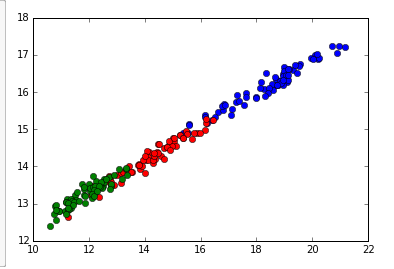
Finally, we can graph the classifications of the data points by the first two features. There are seven features total, but it would be hard to visualize. You can graph by other features for similar visualizations.

# Plot first two features (area vs perimter in this case)
plt.plot(data[cls==0,0], data[cls==0,6],'ob',
        data[cls==1,0], data[cls==1,6],'or',
        data[cls==2,0], data[cls==2,6],'og')
plt.show()

Note: to show the plot inline in the cell, we put ‘%matplotlib inline’ at the beginning of the cell.

Sample Data Here