num2vec: Numerical Embeddings from Deep RNNs

Categories Deep Learning, Machine Learning

Introduction

Encoding numerical inputs for neural networks is difficult because the representation space is very large and there is no easy way to embed numbers into a smaller space without losing information. Some of the ways to currently handle this is:

  • Scale inputs from minimum and maximum values to [-1, 1]
  • One hot for each number
  • One hot for different bins (e.g. [0-0], [1-2], [3-7], [8 – 19], [20, infty])

In small integer number ranges, these methods can work well, but they don’t scale well for wider ranges. In the input scaling approach, precision is lost making it difficult to distinguish between two numbers close in value. For the binning methods, information about the mathematical properties of the numbers such as adjacency and scaling is lost.

The desideratum of our embeddings of numbers to vectors are as follows:

  • able to handle numbers of arbitrary length
  • captures mathematical relationships between numbers (addition, multiplication, etc.)
  • able to model sequences of numbers

In this blog post, we will explore a novel approach for embedding numbers as vectors that include these desideratum.

Approach

My approach for this problem is inspired by word2vec but unlike words which follow the distributional hypothesis, numbers follow the the rules of arithmetic. Instead of finding a “corpus” of numbers to train on, we can generate random arithmetic sequences and have our network “learn” the rules of arithmetic from the generated sequences and as a side effect, be able to encode numbers as vectors and  sequences as vectors.

Problem Statement

Given a sequence of length n integers \(x_1, x_2 \ldots x_n\), predict the next number in the sequence \(x_{n+1}\).

Architecture

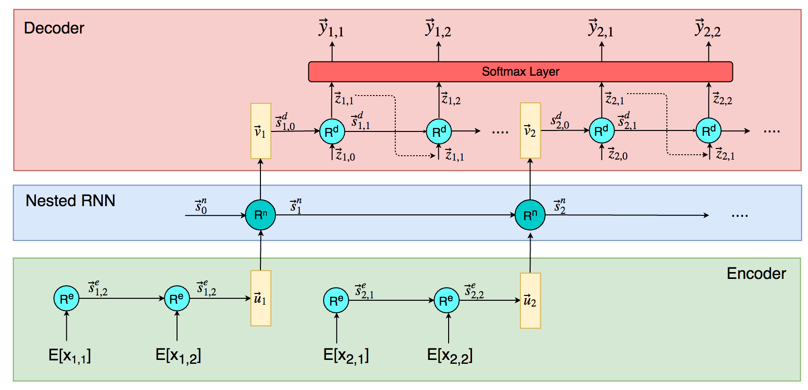
The architecture of the system consists of three parts: the encoder, the decoder and the nested RNN.

The encoder is an RNN that takes a number represented as a sequence of digits and encodes it into a vector that represents an embedded number.

The nested RNN takes the embedded numbers and previous state to output another embedded vector that represents the next number.

The decoder then takes the embedded number and unravels it through the decoder RNN to output the digits of the next predicted number.

Formally:

Let \(X\) represent a sequence of natural numbers where \(X_{i,j}\) represents the j-th digit of the i-th number of the sequence. We also append an <eos> “digit” to the end of each number to signal the end of the number. For the sequence X = 123, 456, 789, we have \(X_{1,2} = 2, X_{3,3} = 9, X_{3,4} = <eos>\).

Let \(l_i\) be the number of digits in the i-th number of the sequence (including <eos> digit. Let \(E\) be an embedding matrix for each digit.

Let \(\vec{u}_i\) be an embedding of the i-th number in a sequence. It is computed as the final state of the encoder. Let \(\vec{v}_i\) be an embedding of the predicted (i+1)-th number in a sequence. It is computed from the output of the nested RNN and used as the initial state of the decoder.

Let \(R^e, R^d, R^n\) be the functions that gives the next state for the encoder, decoder and nested RNN respectively. Let \(O^d, O^n\) be the functions that gives the output of the current state for the decoder and nested RNN respectively.

Let \(\vec{s}^e_{i,j}\) be the state vector for \(R^e\) for the j-th timestep of the i-th number of the sequence. Let \(\vec{s}^d_{i,j}\) be the state vector for \(R^d\) for the j-th timestep of the i-th number of the sequence. Let \(\vec{s}^n_i\) represent the state vector of \(R^n\) for the i-th timestep.

Let \(z_{i,j}\) be the output of \(R^d\) at the j-th timestep of the i-th number of the sequence.

Let \(\hat{y}_{i,j}\) represent the distribution of digits for the prediction of the j-th digit of the (i+1)th number of the sequence.

\(\displaystyle{\begin{eqnarray}\vec{s}^e_{i,j} &=& R^e(E[X_{i,j}], \vec{s}^e_{i, j-1})\\\vec{u}_i &=& \vec{s}^e_{i,l_i}\\ \vec{s}^n_i &=& R^n(\vec{u}_i, \vec{s}^n_{i-1})\\\vec{v_i} &=& O^n(\vec{s}^n_i)\\ \vec{z}_{i,j} &=& O^d(\vec{s}^d_{i,j})\\ \vec{s}^d_{i, j} &=& R^d(\vec{z}_{i,j-1}, \vec{s}^d_{i, j-1})\\ \hat{y}_{i,j} &=& \text{softmax}(\text{MLP}(\vec{z}_{i,j}))\\ p(X_{i+1,j})=k |X_1, \ldots, X_i, X_{i+1, 1}, \ldots X_{i+1, j-1}) &=& \hat{y}_{i,j}[k]\end{eqnarray}}\)

We use a cross-entropy loss function where \(y_{i,j}[t]\) represents the correct digit class for \(y_{i,j}\):

\(\displaystyle{\begin{eqnarray}L(y, \hat{y}) &=& \sum_i \sum_j -\log \hat{y}_{i,j}[t]\end{eqnarray} }\)

Since I also find it difficult to intuitively understand what these sets of equations mean, here is a clearer diagram of the nested network:

Training

The whole network is trained end-to-end by generating random mathematical sequences and predicting the next number in the sequence. The sequences generated contains addition, subtraction, multiplication, division and exponents. The sequences generated also includes repeating series of numbers.

After 10,000 epochs of 500 sequences each, the networks converges and is reasonably able to predict the next number in a sequence. On my Macbook Pro with a Nvidia GT750M, the network implemented on Tensorflow took 1h to train.

Results

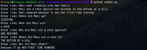
Taking a look at some sample sequences, we can see that the network is reasonably able to predict the next number.

Seq [43424, 43425, 43426, 43427]
Predicted [43423, 43426, 43427, 43428]
Seq [3, 4, 3, 4, 3, 4, 3, 4, 3, 4]
Predicted [9, 5, 4, 3, 4, 3, 4, 3, 4, 3]
Seq [2, 4, 8, 16, 32, 64, 128]
Predicted [4, 8, 16, 32, 64, 128, 256]
Seq [10, 9, 8, 7, 6, 5, 4, 3]
Predicted [20, 10, 10, 60, 4, 4, 3, 2]

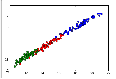
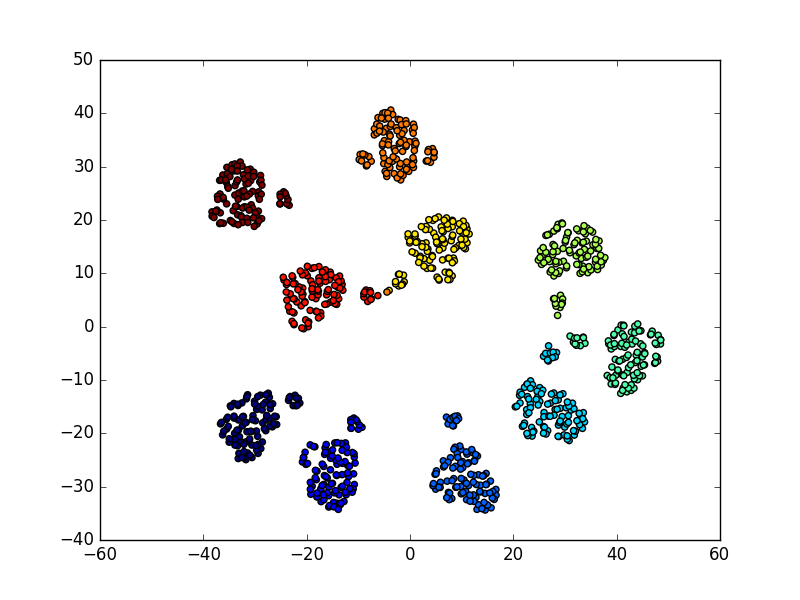
With the trained model, we can compute embeddings of individual numbers and visualize the embeddings with the t-sne algorithm.

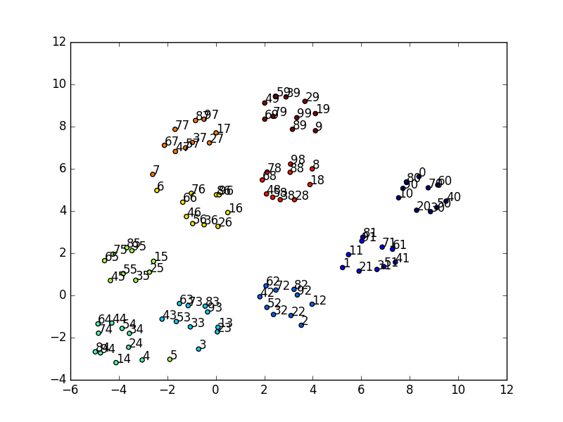
We can see an interesting pattern when we plot the first 100 numbers (color coded by last digit). Another interesting pattern to observe is within clusters, the numbers also rotate clockwise or counterclockwise.

We can also trace the path of the embeddings sequentially, we can see that there is some structure to the positioning of the numbers.

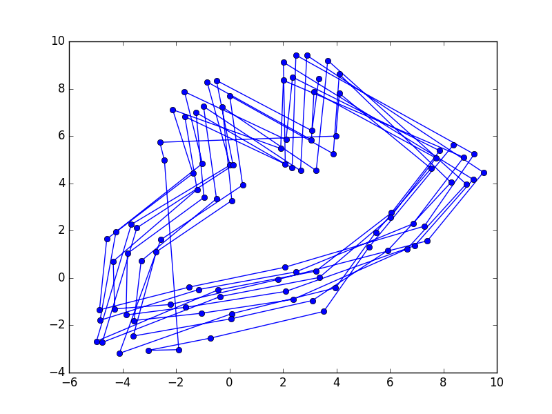
If we look at the visualizations of the embeddings for numbers 1-1000 we can see that the clusters still exist for the last digit (each color corresponds to numbers with the same last digit)

We can also see the same structural lines for the sequential path for numbers 1 to 1000:

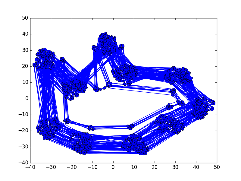
The inner linear pattern is formed from the number 1-99 and the outer linear pattern is formed from the numbers 100-1000.

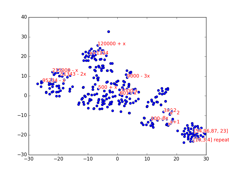
We can also look at the embeddings of each sequence by taking the vector \(\vec{s}^n_k\) after feeding in k=8 numbers of a sequence into the model. We can visualize the sequence embeddings with t-sne using 300 sequences:

From the visualization, we can see that similar sequences are clustered together. For example, repeating patterns, quadratic sequences, linear sequences and large number sequences are grouped together. We can see that the network is able to extract some high level structure for different types of sequences.

Using this, we can see that if we encounter a sequence we can’t determine a pattern for, we can find the nearest sequence embedding to approximate the pattern type.

Code: Github

The model is written in Python using Tensorflow 1.1. The code is not very well written due to the fact that I was forced to use an outdated version of TF with underdeveloped RNN support because of OS X GPU compatibility reasons.

The code is a proof of a concept and comes from the result of stitching together outdated tutorials together.

Further improvements:

  • bilateral RNN
  • stack more layers
  • attention mechanism
  • beam search
  • negative numbers
  • teacher forcing


Stocks with Outperform Ratings Beat the Market

Categories Finance

Introduction

I recently began investing and was wondering how good analysts are at predicting the future of a company. So here is a short data analysis of my curiosity!

In short, we will be answering these hypotheses:

  1. Price targets can accurately reflect the future price of a company.
  2. Some analysts can predict better than others.
  3. A “buy” or “outperform” rating will on average predict a stock moving up.
  4. Some analyst ratings are better than others.
  5. If we were to invest only in stocks with “buy”/”outperform” ratings, we can beat the market.

A price target is the price a financial analyst believes that a stock will reach in a year.

A performance rating is the rating a financial analyst assigns a stock that comes from their combined research and analysis of the company.

Methodology

Since my investments are mostly in Canada, I will be focusing on Canadian equities. To reduce the amount of noise, I looked at companies with the following conditions:

  • Listed on the TSX
  • Market cap over $1 billion
  • Stock price over $5

The source data for companies can be found here: http://www.theupside.ca/list-tsx-stocks-market-capitalization/.

All source code can be found here: http://github.com/ayoungprogrammer/price-targets

Next, to get the price targets and performance ratings, I used Marketbeat and for stock price information, I used the “unofficial” Yahoo Finance api. One restriction is that Marketbeat only had ratings for the last 2 years but it should be enough data to look back at enough ratings.

For each analyst rating assignment, I looked at the 10 day average centered around when it was assigned and the 10 days average centered around a year in time.

After some webscraping and html/json parsing we have the dataframe with sample rows:

ticker analyst target rating aver_close_at_analysis analysis_date aver_close_at_12m 12m_date
0 RY TD Securities 78.00 Hold 70.282856 2016-03-02 97.832857 2017-03-02
1 RY Scotiabank 77.00 Outperform 70.282856 2016-03-02 97.832857 2017-03-02
2 RY TD Securities 80.00 Buy 69.029999 2016-02-25 97.656251 2017-02-25

Each row corresponds to a rating issued by an analyst with the following attributes:

  • ticker: Ticker symbol
  • analyst: Analyst who rated
  • target: Target price issued by analyst
  • rating: Rating issued by analyst
  • aver_close_at_analysis: 10 days average stock price centered on analysis date
  • analysis_date: When the analysis was issued
  • aver_close_at_12m: 10 days average stock price centered 12 months from analysis date
  • 12m_date: 1 year from the analysis date

Results

We can calculate the error between the target price and actual price as follows:

Let

\( t = \) target price,

\(p_0 = \) price at analysis,

\(p_1 = \) price at 12 years after analysis

\(error = 100 \times \frac{t – p_0}{p_0} – \frac{p_1 – p_0}{p_0} \)

Intuitively, this is difference in percentage change from the prediction and the actual. For example, error = 5 means the target price was 5% higher than then actual percentage change.

In code:

df['target_perc'] = (df['target'] - df['aver_close_at_analysis'])/df['aver_close_at_analysis'] * 100
df['real_perc'] = (df['aver_close_at_12m'] - df['aver_close_at_analysis'])/df['aver_close_at_analysis'] * 100
df['error'] = (df['target_perc']-df['real_perc'])
df['abs_error'] = abs(df['error'])
ticker analyst target aver_close_at_12m target_perc real_perc error
0 RY TD Securities 78.00 97.832857 10.980122 39.198750 -28.218627
1 RY Scotiabank 77.00 97.832857 9.557300 39.198750 -29.641449
2 RY TD Securities 80.00 97.656251 15.891643 41.469292 -25.577649

A quick glance at the data shows that some of the ratings have very high variance. Therefore, we should try to reduce the noise of our error measurement by getting rid of some outliers. We will do so by removing outliers in the 10th and 90th percentiles. We also remove analysts with less than 100 ratings, so we can compare the most important analysts.

With pandas, we can easily group the data by analyst and aggregate attributes with different functions:

def filter_tail(data, p1=10, p2=90):
    q1 = np.percentile(data, p1)
    q3 = np.percentile(data, p2)
    return data[(data > q1) & (data < q3)]

analysts = df.groupby(['analyst'], as_index=False)['error'].agg({
        'mean_abs_err': lambda xs:np.mean(np.abs(filter_tail(xs))),
        'count': 'count',
        '10p': lambda xs: np.percentile(xs, q=10),
        '90p': lambda xs: np.percentile(xs, q=90),
        'mean': lambda xs: np.mean(filter_tail(xs)),
        'std': lambda xs: np.std(filter_tail(xs)),
    })
analysts = analysts[analysts['count'] > 100].sort_values(by='mean_no_outliers')
analyst std mean mean_abs_err 10p 90p count
48 National Bank Financial 16.365463 -2.532164 13.425469 -40.092491 30.074729 251
3 BMO Capital Markets 18.982738 -2.282366 14.435614 -55.866637 35.678834 248
7 Barclays PLC 16.120963 -0.586090 13.128664 -35.657920 37.853971 212
20 Desjardins 18.972093 -0.542214 15.355082 -49.563907 33.312509 115
12 Canaccord Genuity 18.101054 4.703447 14.967193 -35.795798 47.363220 302
10 CIBC 19.098723 4.960119 15.799013 -31.113204 48.409297 446
58 Royal Bank of Canada 18.198846 5.544864 15.402881 -34.362247 50.268754 584
66 TD Securities 20.179027 5.868849 17.002451 -44.254427 47.655748 551
54 Raymond James Financial, Inc. 21.500147 7.580748 18.711069 -42.025280 51.284896 269
62 Scotiabank 18.735960 7.741048 15.962621 -32.351408 53.038985 706

We can also plot the means and standard deviations as error plots:

From the aggregate table, we see that Barclays PLC has the least mean absolute error, i.e., its error is closest to 0 and is the most accurate. Barclays PLC also has the “tightest” standard deviation, so it is also the most precise. However, we see that the standard deviations for each analyst is very large; so the precision of each analyst is very low. Barclays PLC has a standard deviation of 16% which we can interpret as 95% of price targets will be +/- 32% off. For example, if TD Bank current stock price is $100 and Barclays PLC gives a price target for $100, all we can reasonably expect is the stock price to range from ~$70 to ~$130.

Thus we can answer our first two hypotheses:

  1. Analysts are on average, accurate in their predictions with their mean error close to 0. However, price targets cannot precisely predict the future of a company in 12 months.
  2. According to the data, Barclays PLC has the most accurate and precise price targets, but only by a small margin.

A more intuitive image of precision vs accuracy:

Next, we will look at analyst ratings and explore their relation to stock performance.

Using pandas again, we can easily filter out price targets with no rating and only take the ratings from analysts that care about (in the previous table). We can also easily group by each analyst and rating and aggregate with different functions on different attribute.

ratings = df[(df['rating'] != 'NaN') & (df['analyst'].isin(analysts['analyst']))]
ratings_agg = ratings.groupby(['analyst', 'rating'], as_index=False).agg({
        'error': {
            'mae': lambda xs: np.mean(np.abs(filter_tail(xs))),
        },
        'real_perc': {
            'mean': 'mean',
            'median': 'median',
            '10p': lambda xs: np.percentile(xs, 10),
            '90p': lambda xs: np.percentile(xs, 90),
            'count': 'count',
        },
        'target_perc': {
            'median': 'median',
            '10p': lambda xs: np.percentile(xs, 10),
            '90p': lambda xs: np.percentile(xs, 90),
        }
    })

ratings_agg.columns = list(map('_'.join, ratings_agg.columns.values))
ratings_agg[ratings_agg['real_perc_count'] > 10]

Attributes:

  • target_perc_10p: 10th percentile for price target change percentage
  • target_perc_90p: 90th percentile for price target change percentage
  • tarc_perc_median: median for perice target change percentage
  • error_mae: mean absolute error
  • real_perc_10p: 10th percentile for real price change percentage
  • real_perc_90p: 90th percentile for real price change percentage
  • real_perc_median: median for real price change percentage
  • real_perc_count: number of ratings
  • real_perc_mean: mean of real price change percentage

Sample rows:

analyst_ rating_ target_perc_10p target_perc_90p target_perc_median error_mae real_perc_10p real_perc_count real_perc_mean real_perc_90p real_perc_median
0 BMO Capital Markets Market Perform -0.249542 23.049416 7.826429 17.048387 -13.624028 82 29.306269 86.571109 11.962594
2 BMO Capital Markets Outperform 9.333289 34.091310 18.863216 13.267287 -13.430220 116 22.215401 64.711223 15.109094
5 Barclays PLC Equal Weight -5.964636 10.834989 4.672844 11.317883 -23.540832 72 11.511754 37.461244 9.239600

Now we take only analyst ratings with at least 20 and then sort by stock performance (change in stock price over a year). We can take the top 10 and perform more analysis on those.

top_ratings = ratings_agg[ratings_agg['real_perc_count'] > 20]
top_ratings = top_ratings.sort_values('real_perc_mean', ascending=False)
top_ratings['analyst_rating'] = top_ratings['analyst_'] + ' ' + top_ratings['rating_']
top_analyst_ratings = top_ratings['analyst_rating'].head(10)
top_analyst_ratings

Sorted by real price change percentage:

analyst_ rating_ target_perc_10p target_perc_90p target_perc_median error_mae real_perc_10p real_perc_count real_perc_mean real_perc_90p real_perc_median analyst_rating
32 National Bank Financial Sector Perform 0.277827 45.337101 8.695651 14.170428 -5.738096 81 29.887596 61.182293 17.410111 National Bank Financial Sector Perform
0 BMO Capital Markets Market Perform -0.249542 23.049416 7.826429 17.048387 -13.624028 82 29.306269 86.571109 11.962594 BMO Capital Markets Market Perform
54 TD Securities Action List Buy 18.333724 77.701954 38.001830 19.629657 -0.893705 36 28.334038 71.459495 15.928740 TD Securities Action List Buy
21 Canaccord Genuity Buy 8.340735 61.226203 24.085974 18.796959 -16.561733 177 27.086690 86.234464 18.039215 Canaccord Genuity Buy
31 National Bank Financial Outperform 7.705539 53.579343 18.929633 12.407454 -1.526925 115 24.524428 59.093628 22.213398 National Bank Financial Outperform
2 BMO Capital Markets Outperform 9.333289 34.091310 18.863216 13.267287 -13.430220 116 22.215401 64.711223 15.109094 BMO Capital Markets Outperform
14 CIBC Sector Outperformer 9.714648 59.846481 33.652243 21.688542 -14.518562 44 22.205022 60.020932 22.218981 CIBC Sector Outperformer
43 Royal Bank of Canada Sector Perform -0.678788 36.516168 11.101983 13.099112 -11.590060 220 21.330160 51.282201 10.498096 Royal Bank of Canada Sector Perform
36 Raymond James Financial, Inc. Outperform 9.437804 54.483693 21.236522 15.914385 -18.695776 106 20.773835 59.159844 13.004491 Raymond James Financial, Inc. Outperform
49 Scotiabank Outperform 7.239955 50.402485 19.082141 15.926344 -21.632875 246 18.407885 51.023159 14.897374 Scotiabank Outperform

We can make an error plot for the mean and standard deviation of the real percentage change for each analyst rating:

We can see that stocks with the top analyst ratings go up on average 25% in a year which is very good. Based on the error plot, TD Security Action List Buy seems to perform the best in terms of high mean and lower variance. Although there is high variance, the mean is more meaningful in this case. If we were to invest $1000 in each of the stocks when were given the rating, we would make about $1250 on average after a year, which is what we really care about. The TSX index went up 11% and TSX index annualized return is 9.1%. So we’re actually beating the market by ~16% with this strategy!

However, keep in mind that this data is for the last 2 years and is not indicative of future performance. On the other hand, I believe this strategy could make sense since analysts put significant effort and research into their rating and also because of the influence of the rating. People probably trust the analysts and would likely invest knowing that the stock has a good rating thus self fulfilling the rating.

With this analysis, we can conclude our last 3 hypotheses:

  1. A buy or outperform rating will on average go up on average by 15-20%.

  2. TD Security Action List Buy appears to be the strongest indicator for a stock to perform well.

  3. If we buy stocks with the top 10 ratings when they get issued and sell in exactly one year, we will beat the market by ~16%.

Conclusion

  • Price targets aren’t a good indicator of where the price of a stock will go.
  • The top performance ratings are a good indicator for a stock performing well.
  • You could possibly beat the market by only buying stocks with sector outperforms or buy ratings and selling in one year.

Please keep in mind that I am by no means a financial expert and am not certified to give financial advice.

All the code can be found here: https://www.github.com/ayoungprogrammer/price-targets

A Natural Language Query Engine without Machine Learning

Categories NLP

What is this?

NLQuery is a natural language engine that will answer questions asked in natural language form.

Demo: http://nlquery.ayoungprogrammer.com

Source: http://ayoungprogrammer.github.com/nlquery

Example:

Input: Who is Obama married to?

Output: Michelle Obama

More examples:

Who is Obama? 44th President of the United States
How tall is Yao Ming? 2.286m
Where was Obama born? Kapiolani Medical Center for Women and Children
When was Obama born? August 04, 1961
Who did Obama marry? Michelle Obama
Who is Obama's wife? Michelle Obama
Who is Barack Obama's wife? Michelle Obama
Who was Malcolm Little known as? Malcolm X
What is the birthday of Obama? August 04, 1961
What religion is Obama? Christianity
Who did Obama marry? Michelle Obama
How many countries are there? 196
Which countries have a population over 1000000000? People's Republic of China, India
Which books are written by Douglas Adams? The Hitchhiker's Guide to the Galaxy, ...
Who was POTUS in 1945? Harry S. Truman
Who was Prime Minister of Canada in 1945? William Lyon Mackenzie King
Who was CEO of Apple Inc in 1980? Steve Jobs

Why no machine learning?

Because a labelled dataset for search queries is hard to find and I wanted to see how well my matching library would work. There are finite amount of grammar rules even though there are an infinite amount of queries and we can build a system that matches these rules. It works surprisingly well and is able to handle many different types of queries, however there were some slight hacks I needed to do handle some queries.

How does it work?

The engine first converts the natural language query to a parse tree, interprets the query into a context and then uses the context to perform a SPARQL query on WikiData. Below is an example of the whole flow:
nlquery

Raw Input

Example of the raw input query string from a user:

"Who is Obama's wife?"

We can do some simple preprocessing to add punctuation and capitalization to the raw input to make it easier to parse in the next step.

Parse Tree

We take the preprocessed string and get the parse tree of the sentence from the Stanford CoreNLP Parser:

(SBARQ
  (WHNP (WP Who))
  (SQ (VBZ is) (NP (NP (NNP Obama) (POS 's)) (NN wife)))
  (. ?))

This parse tree represents the grammatical structure of the sentence and from this we can match the grammar rules to extract the context.

Context

We can convert the grammar parse tree to context parameters by matching the tree with rules. We can doing this using my library for matching parse trees: Lango.

{
    "( SQ ( VP ( VBZ/VBD/VBP:action-o ) ( NP:subj_t ) ) )": {
        subj_t: "( NP ( NP:subject-o ( NNP ) ( POS ) ) ( NN/NNS:prop-o )"
    }
}

This grammar rule matches the parse tree and we can extract some context from the corresponding symbols in the rule.

{
  "prop":"wife",
  "qtype":"who",
  "subject":"obama"
}

We have the subject “Obama”, the property “wife” and the question type “who”. Once we have the contextual parameters of the query, we can construct a SPARQL query to query the WikiData database.

WIkidata SPARQL Query

Wikidata is a free and open knowledge base that can be read and edited by both humans and bots that stores structured data. It uses a graph database to store the data and has an endpoint for a SPARQL graph query. In the high level, entities are represented as nodes and properties of the entities as edges. Every relationship is stored as a triple e.g. (entity:Q76 property:26 entity:13133). This triple represents the relation that entity:Q76 (Obama) has property:26 (spouse) with entity:13133 (Michelle Obama). So if we are querying for the entity that is Obama’s spouse, we are looking for triple of the form (entity:Q76 property:26 ?x) where ?x the unknown entity we are looking for. The SPARQL syntax is beyond the scope of this blog post and if you are interested, you can learn more about the WikiData SPARQL here.

For this application, we will consider two types of SPARQL queries:

  1. finding property of an entity (e.g. Who is Obama’s wife?)
    1. We can search for the property that matches the entity (e.g.entity:Obama property:spouse ?x)
  2. finding instances of entities with given properties (e.g. Which POTUS died from laryngitis?)
    1. We can search for entities that are instances of the type we want that match the properties. E.g. which books are written by Douglas Adams: (?x property:instanceOf entity:book AND ?x property:writtenBy entity:DouglasAdams)
    2. There are some extra cases needed to handle for this such as “positions held” that are a type of entity but is not an instance of. (?x property:positionHeld entity:POTUS AND ?x property:causeOfDeath entity:laryngitis)
Our SPARQL query for the example:
SELECT ?valLabel ?type
WHERE {
{
        wd:Q76 p:P26 ?prop . 
        ?prop ps:P26 ?val .
        OPTIONAL {
            ?prop psv:P26 ?propVal .
            ?propVal rdf:type ?type .
        }
    }
    SERVICE wikibase:label { bd:serviceParam wikibase:language "en"} 
}

 Result

 End result from querying WikiData:

{
    head: {
        vars: [
            "valLabel",
            "type"
        ]
    },
    results: {
        bindings: [
            {
                valLabel: {
                    xml:lang: "en",
                    type: "literal",
                    value: "Michelle Obama"
                }
            }
        ]
    }
}

Thus we get the final answer as “Michelle Obama”.

What else will you add?

Some ideas I have to extend this further would be to:

  • Add other data sources (e.g. DBPedia)
  • Spell check in preprocessing

This is cool! How can I help?

The code is relatively short and simple (~1000 lines with comments) and it should be easy to dive in and make your own pull request!

Natural Language Understanding by Matching Parse Trees

Categories NLP

Natural language understanding is defined as “machine reading comprehension”, i.e., a natural language understanding program can read an English sentence and understand the meaning of it. I have found that a shallow level of understanding can be achieved by matching the parse trees of sentences with only a few rules.

For example, suppose we wish to transform the following sentences into the corresponding programmatic commands:

"Call me an Uber" -> me.call({'item': 'uber'})
"Get my mother some flowers" -> me.mother.get({'item': 'flowers'})
"Order me a pizza with extra cheese" -> me.order({'item': 'pizza', 'with': 'extra cheese'})
"Give Sam's dog a biscuit from Petshop" -> sam.dog.give({'item': 'biscuit', 'from': 'Petshop'})

This seems like a very difficult task, but let’s examine the possible ways we can do this:

1) Use some combination of regexes and conditional statements to match a sentence.
Pros:
  • Simple and easy to implement
  • No data required
Cons:
  • Inflexible model / hard to add more commands
2) Gather hand labelled data of similar sentences and use a machine learning model to predict the intent of the command
Pros:
  • Flexible model / able to generalize
Cons:
  • Requires an abundance of hand labelled data
3) Use intent prediction
Pros:
  • Can use already trained model
  • Easy to use

Cons:

  • Changing model requires adding more data
  • Intent matching is very general
  • Hard to understand what is matched (blackbox)
 
4) Use parse trees to perform rule/pattern based matching

Pros:

  • Simple and easy to implement
  • Easy to modify model
  • More control of what is matched
Cons:
  • Non-adaptive, requires hand matching rules

I believe option 4 is a cheap, quick easy way to get extract meaning from sentences. Many people will argue it’s not “true” AI, but if you’re making a simple bot and not a AI that can philosophize the meaning of life with you, then this is good approach.

Lango

Lango is a natural language library I have created for providing tools for natural language processing.

Lango contains a method for easily matching constituent bracketed parse trees to make extracting information from parse trees easy. A constituent bracketed parse tree is a parse tree in bracketed form that represents the syntax of a sentence.

For example, this is the parse tree for the sentence “Sam ran to his house”:

In a parse tree, the leafs are the words and the other nodes are POS (parts of speech) tags. For example, “to” is a word in the sentence and it is a leaf. It’s parent is the part of speech tag TO (which means TO) and its parent is PP (which is pre-propositional phrase). The list of tags can be found here.

Suppose we want to match the subject (Sam), the action (ran) and the action to the subject (his house).

Let’s first match the top of the parse tree using this match tree:

From the match tree, we get the corresponding matches:
(NP sam) as (NP:subject)
(VBD ran) as (VBD:action)
(PP (TO to) (NP his house)) as (PP:pp)
Our PP subtree looks like:
Now let’s match the PP subtree with this match tree:
From the match tree, we get:
(NP his house) as (NP:to_object)
So the full context match from the two match trees base on this sentence is:
  action: 'ran'
  subject: 'sam'
  to_object: 'his house'
Code to do the matching as described above:
We use the token “NP:to_object-o” to match the tag NP, label it as ‘to_object’ and “-o” means get the string of the tree instead of the tree object.
More explanation of the rule matching syntax/structure can be found on the Github page.

Continue reading “Natural Language Understanding by Matching Parse Trees”

Determining Gender of a Name with 80% Accuracy Using Only Three Features

Categories Uncategorized

Introduction

I thought an easy project to learn machine learning was to guess the gender of a name using characteristics of the name. After playing around with different features by encoding characters of the name, I discovered you only needed THREE features for 80% accuracy which is pretty impressive. I am by no means an expert at machine learning, so if you see any errors, feel free to point them out.

Example:

Name Actual Classified
shea F F
lucero F M
damiyah F F
nitya F F
sloan M M
porter F M
jalaya F F
aubry F F
mamie F F
jair M M

(Click here for Source: IPython Notebook)

Dataset

The dataset used for getting names was from SSN’s baby names dataset for the year 2014.
https://www.ssa.gov/oact/babynames/names.zip

Methodology

I took all the baby names from the dataset that had at least 20 people for male and female since I found many names were low quality when they are least used (for example, there are a few guys named Amy born in 2014).

Loading

Code for loading data from dataset into numpy arrays ready for machine learning

import numpy as np from sklearn.cross_validation
import train_test_split, cross_val_score from sklearn.ensemble
import RandomForestClassifier from sklearn
import svm my_data = np.genfromtxt('names/yob2014.txt', delimiter=',', dtype=[('name','S50'), ('gender','S1'),('count','i4')], converters={0: lambda s:s.lower()})
my_data = np.array([row for row in my_data if row[2]>=20])
name_map = np.vectorize(name_count, otypes=[np.ndarray])
Xlist = name_map(my_data['name'])
X = np.array(Xlist.tolist())
y = my_data['gender']

X is an np.array of N * M, where N is number of names and M is number of features
y is M or F
name_map will be a function that converts a name (string) to an array of features

Fitting and Validation

We will be splitting the data into training and testing for cross-validation and using RandomForrest for classification since it performs well at classifying data.
for x in xrange(5):
 Xtr, Xte, ytr, yte = train_test_split(X, y, test_size=0.33)
 clf = RandomForestClassifier(n_estimators=100, min_samples_split=2)
 clf.fit(Xtr, ytr)
 print np.mean(clf.predict(Xte) == yte)
By default, RandomForest will set max_features(number of features to look at before split) = n_features which is recommended for classification problems (http://scikit-learn.org/stable/modules/ensemble.html#parameters). We will be using n_estimator (number of trees) of 100 and a min_samples_split (the minimum number of samples required to split an internal node) of 2 which we will tune when we determine a good feature set.

Picking Features

Character Frequency

My first attempt at features was the frequency of each character:
def name_count(name):
 arr = np.zeros(52)
 for ind, x in enumerate(name):
 arr[ord(x)-ord('a')] += 1
 return arr
Example:
aaabd
freq: [a:3, b:1, d:1]
* Note that we encode freq as an array using index of letter. e.g.: [3, 1, 0, 1, 0, 0, …. 0]. Most of the array will be zeroes.
Accuracy:
0.690232056125
0.692390717755
0.693739881274
0.688073394495
0.694819212089
Not bad for simple features.

Character Frequency + Order

Second attempt at features is frequency + ordering:
def name_count(name):
 arr = np.zeros(52)
 for ind, x in enumerate(name):
 arr[ord(x)-ord('a')] += 1
 arr[ord(x)-ord('a')+26] += ind+1
 return arr
Example: aaabc
freq: [a:3, b:1, c:1]
ord: [a:6, b:4, c:5]

We can combine these encodings by adding the two arrays together and offsetting the second array

Accuracy:
0.766864543983
0.760388559093
0.766864543983
0.76740420939
0.759848893686
We are getting somewhere!

Character Frequency + Order + 2-grams

Let’s trying adding all the 2-grams in the name as features to see if we can get more info.
def name_count(name):
 arr = np.zeros(52+26*26)
 # Iterate each character
 for ind, x in enumerate(name):
 arr[ord(x)-ord('a')] += 1
 arr[ord(x)-ord('a')+26] += ind+1
 # Iterate every 2 characters
 for x in xrange(len(name)-1):
 ind = (ord(name[x])-ord('a'))*26 + (ord(name[x+1])-ord('a'))
 arr[ind] += 1
 return arr
Example: aaabc
freq: [a:3, b:1, c:1]
ord: [a:6, b:4, c:5]
2-gram: [ aa: 2, ab: 1, bc: 1]
We can encode 2-grams by converting from base 26, e.g.-> aa = 0, bc = 26 + 2 = 28

Accuracy:

0.78548300054
0.771451699946
0.783864004317
0.777388019428
0.77172153265

We get a slight increase in accuracy, but I think we can do better.

Character Frequency + Order + 2-grams + Heuristics

Examining the names more in depth, I hypothesized that the length of name and last and second character of the name could be important.
def name_count(name):
 arr = np.zeros(52+26*26+3)
 # Iterate each character
 for ind, x in enumerate(name):
 arr[ord(x)-ord('a')] += 1
 arr[ord(x)-ord('a')+26] += ind+1
 # Iterate every 2 characters
 for x in xrange(len(name)-1):
 ind = (ord(name[x])-ord('a'))*26 + (ord(name[x+1])-ord('a')) + 52
 arr[ind] += 1
 # Last character
 arr[-3] = ord(name[-1])-ord('a')
 # Second Last character
 arr[-2] = ord(name[-2])-ord('a')
# Length of name
arr[-1] = len(name)
return arr
Example: aaabc
freq: [a:3, b:1, c:1]
ord: [a:6, b:4, c:5]
2-gram: [ aa: 2, ab: 1, bc: 1]
last_char: 3
second_last_char: 2
length: 5
Accuracy:
0.801672962763
0.804641122504
0.803022126282
0.801672962763
0.805450620615

Fine-tuning

After playing around with n_estimators and min_samples_split, I found good values:
clf = RandomForestClassifier(n_estimators=150, min_samples_split=20)
which gives the accuracy:

0.814085267134
0.821370750135
0.818402590394
0.825148407987
0.82245008095

Which gives us a small accuracy increase.

Feature Reduction

Let’s look at the 10 most important features as given by clf.feature_importances:
[728  26 729   0  40  50  30 390  39  37]
[728  26 729  50   0  40  37  30  34 390]
[728  26 729  50  40   0  37  30  39 390]
[728  26 729   0  50  40  30  37 390  39]
[728  26 729   0  50  40  30  37  39  34]

These numbers refer to the feature index by most importance.

728 – Last character
26 – Order of a
729 – Second last character
0 – Number of a’s
50 – order of y

40 – order of o

It looks these 6 features are consistently good.
Let’s see how good the top feature is
def name_count(name):
 arr = np.zeros(1)
 arr[0] = ord(name[-1])-ord('a')+1
 return arr

Accuracy:

0.771451699946
0.7536427415
0.753912574204
0.7536427415
0.760658391797

Wow! We actually get 75% accuracy! This means the last letter of a name is really important in determining the gender.

Let’s take the top three features (last and second last character  and order of a’s) and see the importance of these. (But if you already read the title of this blog post, you should know what to expect.)

def name_count(name):
 arr = np.zeros(3)
 arr[0] = ord(name[-1])-ord('a')+1
 arr[1] = ord(name[-2])-ord('a')+1
 # Order of a's
 for ind, x in enumerate(name):
 if x == 'a':
 arr[2] += ind+1
 return arr

Accuracy:

0.798165137615
0.794117647059
0.795736643281
0.801133297356
0.803561791689

I would say 80% accuracy for 3 features is pretty good for determining gender of a name. Thats about the same accuracy as a mammogram detecting cancer in a 45-49 year old woman!

Sample Example

We can sample random datapoints to see how well our model is performing:
def name_count(name):
 arr = np.zeros(3)
 arr[0] = ord(name[-1])-ord('a')+1
 arr[1] = ord(name[-2])-ord('a')+1
 # Order of a's
 for ind, x in enumerate(name):
 if x == 'a':
 arr[2] += ind+1
 
 return arr

my_data = np.genfromtxt('names/yob2014.txt', 
 delimiter=',', 
 dtype=[('name','S50'), ('gender','S1'),('count','i4')],
 converters={0: lambda s:s.lower()})
my_data = np.array([row for row in my_data if row[2]>=20])
name_map = np.vectorize(name_count, otypes=[np.ndarray])
Xname = my_data['name']
Xlist = name_map(Xname)
X = np.array(Xlist.tolist())

y = my_data['gender']

Xtr, Xte, ytr, yte = train_test_split(X, y, test_size=0.33)
clf = RandomForestClassifier(n_estimators=150, min_samples_split=20)
clf.fit(Xtr, ytr)

idx = np.random.choice(np.arange(len(Xlist)), 10, replace=False)
xs = Xname[idx]
ys = y[idx]
pred = clf.predict(X[idx])

for a,b, p in zip(xs,ys, pred):
 print a,b, p

Output:

Name Actual Classified
shea F F
lucero F M
damiyah F F
nitya F F
sloan M M
porter F M
jalaya F F
aubry F F
mamie F F
jair M M

Conclusion

Many features are good, but finding important features is better.
If you are unsure of a gender of a name, just look at the last letter which gives you a 75% chance of getting it.

I hope you have learned something from reading this blog post as I did writing it!(Click here for Source: IPython Notebook)

Tutorial: Getting Started with Distributed Deep Learning with Caffe on Windows

Categories Machine Learning, Uncategorized

Introduction

What is Caffe?

A deep learning framework developed by Berkeley Vision and Learning Center. It makes creating deep neural networks easy without writing a ton of code.If you don’t know what deep learning is, here is a great guide to getting started: http://cs231n.github.io/.

Setup

My setup:
Windows 8.1 on 64bit
Visual Studio 2013 Community
GeForce GT 750M
CUDA 7.5

1. Check for Compatibility

Make sure you are on a supported Windows operating system:
Windows 8.1
Windows 7
Windows Server 2008
Windows Server 2012.(If you are using Windows 8, upgrade through here: http://windows.microsoft.com/en-ca/windows-8/update-from-windows-8-tutorial)

Make sure your GPU is supported by CUDA: https://developer.nvidia.com/cuda-gpus 
Anything with compute capability of  >=3.0 should be good.

If you do not have a compatible GPU, you can still use Caffe but it will be magnitudes slower than with a GPU and skip part 2.

Make sure you have a compatible Visual Studios for CUDA support: 
Visual Studio 2013
Visual Studio 2013 Community (Download Visual Studio 2013 Community Edition Free)
Visual Studio 2012
Visual Studio 2010

More nVidia documentation at:
http://docs.nvidia.com/cuda/cuda-getting-started-guide-for-microsoft-windows/#axzz3wsl3JktL 

2. Install CUDA

Download and install CUDA toolkit here: https://developer.nvidia.com/cuda-downloads
 
Verify CUDA can compile:
Go to C:ProgramDataNVIDIA CorporationCUDA Samplesv7.5 and open the solution file (i.e. Samples_vs2013.sln) in Visual Studio
In the solution explorer, build 0_Simple/vectorAdd
Run C:ProgramDataNVIDIA CorporationCUDA Samplesv7.5binwin64debugvectorAdd.exe
 
The output should be:
Copy input data from the host memory to the CUDA device
CUDA kernel launch with 196 blocks of 256 threads
Copy output data from the CUDA device to the host memory
Test PASSED
Done

3. Install Caffe

Fork the windows port of Caffe: https://github.com/happynear/caffe-windowsDownload third party libraries and extract to caffe-windows/3rdparty
Remember to add caffe-windows/3rdparty/bin to your PATH

Open caffe-windows/buildVS2013/MainBuilder.sln in Visual Studio
If you don’t have a compatible GPU, open caffe-windows/build_cpu_only/MainBuilder.sln

Set the GPU compatible mode:
Right click the caffe project and click properties
In the left menu, go to Configuration Properties -> Cuda C/C++ -> Device
In the Code Generation key, modify the compute capabilities to your GPU’s (such as compute_30,sm_30; etc)

Build the solution in release mode
Right click the solution and click Build Solution
(It’s OK if matcafe and pycafe fail)

Testing
Download the mnist leveldb from http://pan.baidu.com/s/1mgl9ndu
Extract the folders to caffe-windows/examples/mnist
Run caffe-windows/run_mnist.bat

You should get some output similar to the following when you finish:
….
I0112 00:06:37.180341 45040 solver.cpp:326] Iteration 10000, loss = 0.00428135
I0112 00:06:37.181342 45040 solver.cpp:346] Iteration 10000, Testing net (#0)
I0112 00:06:51.726634 45040 solver.cpp:414]     Test net output #0: accuracy = 0
.9914
I0112 00:06:51.726634 45040 solver.cpp:414]     Test net output #1: loss = 0.027
0199 (* 1 = 0.0270199 loss)
I0112 00:06:51.726634 45040 solver.cpp:331] Optimization Done.
I0112 00:06:51.726634 45040 caffe.cpp:215] Optimization Done.

Full instructions can be found on the readme of https://github.com/happynear/caffe-windows

Results:
solver_mode: GPU
Start Time: 23:25:19.38
Finish Time: 23:28:37.62

solver_mode: CPU

Start Time: 23:38:01.62
Finish Time:  0:06:51.91As you can see, even a low-end GPU can train a magnitude faster than a CPU.

A Simple Artificial Intelligence Capable of Basic Reading Comprehension

Categories Machine Learning, Uncategorized
I was interested in an artificial intelligence that could do reading comprehension, but surprisingly,  I could not find much on the topic. I decided to try and create an AI that could do some basic reading comprehension and I got some good results:

Short Passage (Input):
Mary went sledding with her family. Mary won a race against her brother to the bottom of a hill. Mary cheered because it was her first time winning.

Input: Where did Mary go?
Output: Sledding

Input: What did Mary win?
Output: A race


Input: Who did Mary win a race against?
Output: Her brother

Input: Where did Mary win a race to?
Output: The bottom of the hill


Input: Why did Mary cheer?
Output: Because it was her first time winning


As we can see, the program can actually answer the questions about the passage.

Full Source Available Here

Introduction

What I am trying to accomplish is program capable of artificial semantic memory. Semantic memory refers to how we store our explicit knowledge and facts about the world. For example, our memory of our birth date or our knowledge that humans are mammals. I wanted to be able to make something that was able to read a passage and answer any questions I had.

Abstract Idea

An abstract idea of how I accomplished artificial semantic memory was to create a structure that can store a sentence in a different way that can be used to answer questions.

1. Structure the relationships betweens objects (nouns) in the sentence.

For example, in the sentence “Mary went sledding with her family”, there are three objects “Mary”, “sledding” and “her family”. Mary has a verb “go” (present tense of went) with the object “sledding”. The verb “go” is “with” the object “her parents”. 
After brainstorming different ways to represent the relationships between objects and actions, I came up with a structure similar to a trie which I will call a “word graph”. In a word graph, each word is a node and the edges are actions or propositions. 
Examples:
Mary went sledding with her family
Mary won a race against her brother to the bottom of the hill
Mary cheered because it was her first time winning

2. Answer questions using the structure.

A key observation to answering questions is that they can be reworded to be fill in the blanks. 
Examples:
Where did Mary go -> Mary went _______
What did Mary win -> Mary won _______
Who did Mary win a race against? -> Mary won a race against _______
Why did Mary cheer -> Mary cheered because/since _______
We can use this observation to read out answers from our tree structure. We can parse the question, convert it to a fill in the blank format and then 
Example:
Mary went _____
By following the tree, we see that we should put “sledding” in the blank.
Mary won _______
Mary won a race against ______
Mary won a race to ______
By following the tree, we see that Mary won “a race”, against “her brother”, to “the bottom”.

Implementation

I chose to implement this in Python since it is easy to use and has libraries to support natural language processing. There are three steps in my program: parsing, describing and answering. 
Parsing converting a sentence to a structure that makes sense of the sentence structure.
Describing is reading in a sentence and adding the information to our tree structure.
Answering is reading in a question, changing the format and completing from our tree structure.

Parsing

The first thing we have to do is parse the sentence to see the sentence structure and to determine which parts of a sentence are objects, verbs and propositions. To do this, I used the Stanford parser which works well enough for most cases. 
Example: the sentence “Mary went sledding with her family” becomes:
  (S
    (NP (NNP Mary))
    (VP
      (VBD went)
      (NP (NN sledding))
      (PP (IN with) (NP (PRP$ her) (NN family)))))
The top level tree S (declarative clause) has two children, NP (noun phrase) and VP (verb phrase). The NP consist of one child NNP (proper noun singular) which is “Mary”. The VP has three children: VBD (verb past tense) which is “went”, NP, and a PP (propositional phrase). We can use the recursive structure of a parse tree to help us build our word graph.

A full reference for the parsers tags can be found here.

I put the Stanford parser files in my working directory but you might want to change the location to where you put the files.

os.environ['STANFORD_PARSER'] = '.'
os.environ['STANFORD_MODELS'] = '.'

parser = stanford.StanfordParser()

line = 'Mary went sledding with her family'
tree = list(parser.raw_parse(line))[0]

Describing

We can use the parse tree to build the word graph by doing it recursively. For each grammar rule, we need to describe how to build the word graph.

Our method looks like this:

# Returns edge, node 
def describe(parse_tree):

 ...

  if matches(parse_tree,'( S ( NP ) ( VP ) )'):

    np = parse_tree[0] # subject
    vp = parse_tree[1] # action

    _, subject = describe(np) # describe noun
    action, action_node = describe(vp) # recursively describe action

    subject.set(action, action_node) # create new edge labeled action to the action_node
    return action, action_node

  ....
We do this for each grammar rule to recursively build the word graph. When we see a NP (noun phrase) we treat it as an object and extract the words from it. When we see a proposition or verb, we attach it to the current node and when we see another object, we use a dot ( . ) edge to indicate the object of the current node.

Currently, my program supports the following rules:

( S ( NP ) ( VP ) )
( S ( VP ) )
( NP )
( PP ( . ) ( NP ) )
( PRT )
( VP ( VBD ) ( VP ) $ )
( VP ( VB/VBD ) $ )
( VP ( VB/VBZ/VBP/VPZ/VBD/VBG/VBN ) ( PP ) )
( VP ( VB/VBZ/VBP/VPZ/VBD/VBG/VBN ) ( PRT ) ( NP ) )
( VP ( VB/VBZ/VBP/VPZ/VBD/VBG/VBN ) ( NP ) )
( VP ( VB/VBZ/VBP/VPZ/VBD/VBG/VBN ) ( NP ) ( PP ) )
( VP ( VB/VBZ/VBP/VPZ/VBD/VBG ) ( S ) )
( VP ( TO ) ( VP ) )
( VP ( VB/VBZ/VBP/VPZ/VBD/VBG/VBN ) ( ADJP ) )
( VP ( VB/VBZ/VBP/VPZ/VBD/VBG/VBN ) ( SBAR ) )
( SBAR ( IN ) ( S ) )

For verbs, I used Nodebox (a linguistic library) for getting the present tense of a word so that the program knows different tenses of a word. E.g. “go” is the same word as “went”. 

Answering

We can answer questions by converting the question to a “fill in the blank” and then following the words in the “fill in the blank” in the word graph to the answer. My program supports two types of fill in the blanks: from the end and from the beginning.

Type I: From the end

A from the end type of fill in the blank is a question like:

Where did Mary go?

Which converts to:

Mary went _______

And as you can see, the blank comes at the end of the sentence. We can fill in this blank by following each word in our structure to the answer. A sample of the code is below:

# Matches "Where did Mary go"
if matches(parse_tree, '( SBARQ ( WHADVP ) ( SQ ( VBD ) ( NP ) ( VP )  )'):

  tokens = get_tokens(parse_tree) # Get tokens from parse tree

  subject = get_node(tokens[3]) # Get subject of sentence

  tokens = tokens[3:] # Skip first two tokens to make fill in the blank

  return subject.complete(tokens) # Complete rest of tokens
The node completes by reading each token and following the corresponding edges. When we run out of tokens, we follow the first edge until we reach another object and return the edges followed and the object.

Simplified node.complete:

class Node:
  ...
  def complete(self, tokens, qtype):
    if len(tokens) == 0:
      # no tokens left
      if qtype == 'why':
        # special case
        return self.why()
      if self.isObject:
        # return object
        return self.label
      else:
        # follow first until object
        return self.first.label + self.first.complete(tokens, qtype) 
    else:
      for edge, node in self:
        if edge == tokens[0]:
          # match rest of tokens
          return node.complete(tokens, qtype) 
      return "No answer"
  ...

We have to handle “Why” as a special case because we need to complete with “because” or “since” after there are no more tokens and we have to iterate backwards to the first object.

Type 2: From the beginning

A from the beginning type is a question like:

Who went sledding?

Which converts to:

 ____ went sledding?

As we can see, the blank is at the beginning of the sentence and my solution for this was to iterate through all possible objects and see which objects have tokens that match the rest of the fill in the bank.

Further Steps

There is still a long way to go, to make an AI perform reading comprehension at a human level. Below are some possible improvements and things to handle to make the program better:

Grouped Objects

We need to be able to handle groups of objects, e.g. “Sarah and Sam walked to the beach” should be split into two individual sentences.

Pronoun Resolution

Currently, pronouns such as he and she are not supported and resolution can be added by looking at the last object. However, resolution is not possible in all cases when there are ambiguities such as “Sam kicked Paul because he was stupid”. In this sentence “he” could refer to Sam or Paul.

Synonyms

If we have the sentence: “Jack leaped over the fence”, the program will not be able to answer “What did Jack jump over” since the program interprets jump as a different word than leap. However, we can solve this problem by using asking the same question for all synonyms of the verb and seeing if any answers work.

Augmented Information

If we have the sentence “Jack threw the football to Sam”, the program would not be able to answer “Who caught the football”. We can add information such as “Sam caught the football from Jack” which we can infer from the original sentence.

Aliasing

Sometimes objects can have different names, e.g. “James’s dog is called Spot” and the program should be able to know that James’ dog and Spot both refer to the same object. We can do this by adding a special rule for words such as “called”, “named”, “also known as” , etc.

Other

There are probably other quirks of language that need to be handled and perhaps instead of explicitly handling all these cases, we should come up with a machine learning model that can read many passages and be able to construct a structure of the content as well as to augment any additional information.

Full Source Available Here

Tutorial: Getting Started with Machine Learning with the SciPy stack

Categories Machine Learning, Uncategorized
There are many machine learning libraries out there, but I heard that SciPy was good so I decided to try it out. We will be doing a simple walkthrough a k means clustering example:

Full Source Here


Sample Data Here

SciPy Stack

The contents of the SciPy stack are:

Python: Powerful scripting language
Numpy: Python package for numerical computing
SciPy: Python package for scientific computing
Matplotlib: Python package for plotting
iPython: Interactive python shell
Pandas: Python package for data analysis
SymPy: Python package for computer algebra systems
Nose: Python package for unit tests

Installation

I will go through my Mac installation but if you are using another OS, you can find the installation instructions for SciPy on: http://www.scipy.org/install.html.

You should have Python 2.7.

Mac Installation

I am using a Mac on OS X 10.8.5 and used MacPorts to setup the SciPy stack on my machine.

Install macports if you haven’t already: http://www.macports.org/

Otherwise open Terminal and run: ‘sudo macports selfupdate’

Next in your Terminal run: ‘sudo port install py27-numpy py27-scipy py27-matplotlib py27-ipython +notebook py27-pandas py27-sympy py27-nose’

Run the following in terminal to select package versions.

sudo port select –set python python27
sudo port select –set ipython ipython27

Hello World

IPython allows you to create interactive python notebooks in your browser. We will get started by creating a simple hello world notebook.
Create a new directory where you want your notebooks to be placed in.
In your directory, run in terminal:
ipython notebook

This should open your browser to the IPython notebook web interface. If it does not open, point your browser to http://localhost:8888.

 Click New -> Notebooks -> Python 2


This should open a new tab with a newly create notebook.

Click Untitled at the top, rename the notebook to Hello World and press OK.

In the first line, change the line format from Code to Markdown and type in:

# Hello World Code

And click run (the black triangle that looks like a play button)

On the next line, in code, type:

print ‘Hello World’

and press run.

K Means Clustering Seed Example

Suppose we are doing a study on a wheat farm to determine how much of each kind of wheat is in the field. We collect a random sample of seeds from the field and measure different attributes such as area, perimeter, length, width, etc. Using this attributes we can use k-means clustering to classify seeds into different types and determine the percentage of each type.

Sample data can be found here: http://archive.ics.uci.edu/ml/datasets/seeds

The sample data contains data that comes from real measurements. The attributes are:

1. area A, 
2. perimeter P, 
3. compactness C = 4*pi*A/P^2, 
4. length of kernel, 
5. width of kernel, 
6. asymmetry coefficient 
7. length of kernel groove. 

Example: 15.26, 14.84, 0.871, 5.763, 3.312, 2.221, 5.22, 1

Download the file into the same folder as your notebook.

Code

Create a new notebook and name it whatever you want. We can put all the code into one cell.

First, we need to parse the data so that we can run k-means on it. We open the file using a csv reader and convert each cell to a float. We will skip rows that contain missing data.

Sample row:

['15.26', '14.84', '0.871', '5.763', '3.312', '2.221', '5.22', '1']
# Read data
for row in bank_csv:
    missing = False
    float_arr = []
    for cell in row:
        if not cell:
            missing = True
            break
        else:
            # Convert each cell to float
            float_arr.append(float(cell))
    # Take row if row is not missing data
    if not missing:
        data.append(float_arr)
data = np.array(data)

Next, we normalize the features for the k means algorithm. Since Scipy implements the k means clustering algorithm for us, all the hard work is done.

# Normalize vectors
whitened = vq.whiten(data)

# Perform k means on all features to classify into 3 groups
centroids, _ = vq.kmeans(whitened, 3)

We then classify each data point by distance to centroid:

# Classify data by distance to centroids
cls, _ = vq.vq(whitened, centroids)

Finally, we can graph the classifications of the data points by the first two features. There are seven features total, but it would be hard to visualize. You can graph by other features for similar visualizations.

# Plot first two features (area vs perimter in this case)
plt.plot(data[cls==0,0], data[cls==0,6],'ob',
        data[cls==1,0], data[cls==1,6],'or',
        data[cls==2,0], data[cls==2,6],'og')
plt.show()

Note: to show the plot inline in the cell, we put ‘%matplotlib inline’ at the beginning of the cell.

Sample Data Here

Using an Arduino Uno as a Spotify Controller on Mac

Categories Uncategorized
I recently bough an Arduino Uno with a 1.8″ TFT Arduino Shield and I thought I would have some fun with it by using it as a Spotify controller.

Hardware:
Arduino Uno
Adafruit 1.8″ TFT Shield

Software:
Mac OS X 10.8.5 Mountain Lion
rb-appscript 0.6.1
Ruby

There are three steps to this project:

  1. Interact with Spotify and be able to get the artist and song as well as perform actions such as next track, previous track, play/pause, increase volume and decrease volume.
  2. Use the serial port through USB to send data between Arduino and Mac.
  3. Display song, artist and use joystick input for controls.

Step 1: Interact with Spotify

The Mac version of Spotify supports Applescript so we can use that to perform the actions we need. However, I wanted to keep all the app code in the same language (Ruby) and in the same script so I found a gem (rb-applescript) that executes Applescript with Ruby.

Install rb-applescript
gem install rb-applescript

For example:
 require 'appscript'  
   
 spot = Appscript.app('Spotify')  
 spot.launch  
   
 # Get track info  
 artist = spot.current_track.artist.get  
 song = spot.current_track.name.get  
   
 # Toggle play/pause  
 spot.playpause  
   
 # Play next track  
 spot.previous_track  
   
 # Play next track  
 spot.next_track  
   
 # Get volume  
 curVol = spot.sound_volume.get  
   
 # Decrease volume  
 spot.sound_volume.set(curVol - 10)  
   
 # Increase volume  
 spot.sound_volume.set(curVol + 10)  
   

Step 2: Use Serial Port with Arduino

Ruby has a serial port gem that allows you to read/write from the serial port to your Arduino:

gem install serialport

Example:

 # Gem for serial port IO  
 require 'serialport'  
   
 # Include Input stream ready?  
 require 'io/wait'  
   
 # Open serial port to your port location  
 sp = SerialPort.new("/dev/cu.usbmodem411", 9600)  
   
 # Write to serial port  
 sp.write("hellon")  
   
 # Nonblocking read from serial   
 while true  
  # Other actions...  
   
  # Nonblocking input  
  if sp.ready?  
   # Get string and chomp rn from end of string  
   str = sp.gets.chomp  
   puts str
  end

The Arduino Uno can also send and receive from USB port:

 // Input from serial port  
 if(Serial.available() > 0){  
  String data = Serial.readString();  
 }  
 // Output to serial port  
 Serial.println("output");  

Step 3: Display with Arduino and read Joystick

The 1.8″ TFT Shield I bought from Adafruit came with a graphics library for drawing shapes and text. We can use it to draw the current song and track to the screen.

 void printArtist(uint16_t color) {  
  tft.setCursor(0, 0);  
  tft.setTextSize(2);  
  tft.setTextColor(color);  
  tft.setTextWrap(false);  
  tft.print(artist);  
 }  
 void printSong(uint16_t color) {  
  tft.setCursor(x, 50);  
  tft.setTextSize(2);  
  tft.setTextColor(color);  
  tft.setTextWrap(false);  
  tft.print(song);  
 }  

Since the screen is not wide enough to display a full song name, we will animate the song text by scrolling to the left. We will do this by redrawing the song name X units to the left every 0.5 seconds where X is determined by the desired scroll speed. When we redraw, we draw the song text of the previous position in the background color and then we draw the song text again in the text color shifted X units left. We do this because we want to minimize the number of pixel draws since redrawing the screen causes a flicker. When the end of the song name reaches the screen, we need to reset it back to the original position. The width of each character in text size 2 is 12 pixels and the screen width is 128 pixels so if x < -12 *song.length() + 128, we reset x.

In our loop() function:

 if(time + 500 < millis()) {  
  time = millis();  
  printSong(ST7735_BLACK);  
  x -= SCROLL;  
  if(x < (-12 * (int)song.length() + 128)){  
   x = SCROLL;  
  }  
  printSong(ST7735_BLUE);  
 }  

The joystick can be read by reading analog 3.

 #define Neutral 0  
 #define Press 1  
 #define Up 2  
 #define Down 3  
 #define Right 4  
 #define Left 5  
 int CheckJoystick(){  
  int joystickState = analogRead(3);  
  if (joystickState < 50) return Left;  
  if (joystickState < 150) return Down;  
  if (joystickState < 250) return Press;  
  if (joystickState < 500) return Right;  
  if (joystickState < 650) return Up;  
  return Neutral;  
 }  

We only send the state of the joystick if it changes:

 int curCmd = CheckJoystick();  
  if(curCmd != lastCmd){  
  Serial.println(curCmd);  
  lastCmd = curCmd;  
 }  

In our ruby app, we can perform actions based on the joystick state.

Putting it all together:

https://github.com/ayoungprogrammer/arduino-spotify-controller

The Computer Science Handbook – A Reference for Algorithms and Data Structures

Categories Uncategorized
I’ve been working on this site that teaches algorithms and data structures in a way that doesn’t require a strong math background. It’s meant for supplementary material for university courses, reviewing for job interviews or an everyday day reference. Please check it out and I hope you find it helpful in your future endeavors!